Pandas is a Python package built to work with spreadsheet-like data, and it is very good at its job. Pandas stores data in something called a “dataframe”. A dataframe is simply data stored in rows and columns. As an example, here is some sample data taken by an accelerometer sitting on an elevator floor:
Every dataframe has labels attached to its columns and rows. In this example, the row labels are just the first 10 integers and the column labels are “time”, “gFx”, “gFy”, and , “gFz”. Labeling the rows and columns is nice because you can access data using the row and column labels instead of indices.
13.1 Creating dataframes
A dataframe can be initiated in many ways but the most common are: from file, from a dictionary, and from an array or list. We’ll discuss each way separately.
13.1.1 Reading from a .csv file.
The most-used function from the pandas module is read_csv which is used to read a csv-formatted file into a data frame. To use it, simply call the pandas.read_csv function and pass in the path to the .csv file. (Here is a link to the file.)
from pandas import read_csvelevator_data = read_csv("elevator.csv",index_col =0)print(elevator_data)
The keyword argument index_col = 0 indicates that the row labels should be taken from the first column in the csv file. There are many, many possible keyword arguments that can be used to customize the way read_csv reads a file into a dataframe. I’ll highlight just a few and refer you to the documentation for the rest:
delimiter- use this to specify the character that separates the data from each other. The default is “,” for .csv files.
header - use this to specify which row contains the column names. Usually this occurs on the first row (header = 0) but not always.
usecols - use this to specify which columns from the file should be included in the dataframe.
skiprows - line numbers to skip when building the dataframe. Can be either a single integer (skip the first n lines) or a list of integers and it will skip all rows in the list.
The rename() function can be used if you don’t like the default index values (integers if you read from file) and want to reassign them.
    time     gFx     gFy     gFz
A  0.007 -0.0056 -0.0046  1.0120
B  0.008  0.0070  0.0024  1.0022
C  0.008  0.0000  0.0059  1.0039
D  0.009  0.0054 -0.0022  1.0032
E  0.009 -0.0015 -0.0056  1.0042
F  0.009  0.0037 -0.0020  0.9951
G  0.010 -0.0020 -0.0020  1.0020
H  0.014  0.0090 -0.0025  1.0159
I  0.015  0.0012 -0.0037  1.0100
J  0.017 -0.0115 -0.0020  1.0012
13.1.2 Create from a dictionary
If your data is in a dictionary you can use the DataFrame function (case sensitive) to initialize the dataframe. Key values in the dictionary correspond to columns in the dataframe.
from pandas import DataFrameelevator = {"time":[0.007,0.008,0.008,0.009,0.009,0.009,0.01,0.014,0.015,0.017],"gFx":[-0.0056,0.007,0,0.0054,-0.0015,0.0037,-0.002,0.009,0.0012,-0.0115],"gFy":[-0.0046,0.0024,0.0059,-0.0022,-0.0056,-0.002,-0.002,-0.0025,-0.0037,-0.002],"gFz":[1.012,1.0022,1.0039,1.0032,1.0042,0.9951,1.002,1.0159,1.01,1.0012]}elevator_data = DataFrame(elevator)print(elevator_data)
The row indices will default to the a set of integers starting at 0. If you want to index the rows with other labels, use the index keyword argument.
from pandas import DataFrameelevator = {"time":[0.007,0.008,0.008,0.009,0.009,0.009,0.01,0.014,0.015,0.017],"gFx":[-0.0056,0.007,0,0.0054,-0.0015,0.0037,-0.002,0.009,0.0012,-0.0115],"gFy":[-0.0046,0.0024,0.0059,-0.0022,-0.0056,-0.002,-0.002,-0.0025,-0.0037,-0.002],"gFz":[1.012,1.0022,1.0039,1.0032,1.0042,0.9951,1.002,1.0159,1.01,1.0012]}elevator_data = DataFrame(elevator,index = ["A","B","C","D","E","F","G","H","J","K"])print(elevator_data)
    time     gFx     gFy     gFz
A  0.007 -0.0056 -0.0046  1.0120
B  0.008  0.0070  0.0024  1.0022
C  0.008  0.0000  0.0059  1.0039
D  0.009  0.0054 -0.0022  1.0032
E  0.009 -0.0015 -0.0056  1.0042
F  0.009  0.0037 -0.0020  0.9951
G  0.010 -0.0020 -0.0020  1.0020
H  0.014  0.0090 -0.0025  1.0159
J  0.015  0.0012 -0.0037  1.0100
K  0.017 -0.0115 -0.0020  1.0012
13.1.3 Create from a list
Sometimes you have data in a list or multiple list and would like to combine all of that data and form a dataframe. This can also be done using the DataFrame function (case sensitive remember!). When initializing with lists, you have to also use the columns keyword argument to specify what you want the column labels to be.
Extracting data from the dataframe could mean several things. The most common possibilities include:
accessing a single number using row and column labels or row and column indices.
accessing one or several columns of the dataframe.
accessing one or several rows of the dataframe.
slicing from the “middle” of the dataframe. (i.e. Not entire columns or entire rows.)
accessing only elements in the dataframe that meet a certain criteria.
We’ll cover each of these tasks one at a time.
13.2.1 Extracting General Information
Sometimes the dataframe is quite large and you’d like to inspect just a small portion of it. You can use dataframe.head(n) to look at the firstn rows in the dataframe and dataframe.tail(n) to look at the lastn rows.
elevator_data.head(3)elevator_data.tail(4)
time
gFx
gFy
gFz
G
0.010
-0.0020
-0.0020
1.0020
H
0.014
0.0090
-0.0025
1.0159
J
0.015
0.0012
-0.0037
1.0100
K
0.017
-0.0115
-0.0020
1.0012
To get a list of the column or row labels, use the variables dataframe.columns and dataframe.index.
To extract a single number from a dataframe, use the dataframe.at[] or dataframe.iat[] objects. The at object should be used if you want to locate the number using row and column labels and iat should be used when you want to access the number using row and column indices. Let’s see an example:
You can bundle the column names into a list and extract multiple columns at once.
elevator_data[["gFx", "gFy", "gFz"]]
13.2.4 Accessing entire rows
Accessing rows in a dataframe is done with the help of the dataframe.loc[n] or dataframe.iloc[n] dictionary. loc should be used if you want to slice using row and column labels whereas iloc should be used if you want to slice out using indices.
We have already seen boolean slicing in Numpy Arrays and we can use something similar on Pandas. Let’s see an example:
from pandas import DataFramefrom numpy import transposetime = [0.007,0.008,0.008,0.009,0.009,0.009,0.01,0.014,0.015,0.017]gFx = [-0.0056,0.007,0,0.0054,-0.0015,0.0037,-0.002,0.009,0.0012,-0.0115]gFy = [-0.0046,0.0024,0.0059,-0.0022,-0.0056,-0.002,-0.002,-0.0025,-0.0037,-0.002]gFz = [1.012,1.0022,1.0039,1.0032,1.0042,0.9951,1.002,1.0159,1.01,1.0012]elevator_data = DataFrame(transpose([time,gFx,gFy,gFz]),columns = ["time", "gFx","gFy", "gFz"],index = ["A","B","C","D","E","F","G","H","J","K"])elevator_data[elevator_data["time"] <0.01] # Slice only the rows where time < 0.01
time
gFx
gFy
gFz
A
0.007
-0.0056
-0.0046
1.0120
B
0.008
0.0070
0.0024
1.0022
C
0.008
0.0000
0.0059
1.0039
D
0.009
0.0054
-0.0022
1.0032
E
0.009
-0.0015
-0.0056
1.0042
F
0.009
0.0037
-0.0020
0.9951
The statement elevator_data["time"] < 0.01 produces a boolean sequence which can be used as a set of indices to access only those entries where time is less than 0.01.
More complex boolean slicing can be done with the use of the query function which allows you to be more specific about your boolean conditions. The example below will extract all rows in the dataframe where time > 0.008 and gFz is greater than 1.
Often you will find that your column labels will contain spaces and/or other special characters in them. To correctly specify the column label in these cases, you must enclose the name in graves accents (It’s located above the tab key on your keyboard.). For example, if your column label was ” time-s” instead of just “time” like in the example above, you could use the query function like this:
Often your dataframe will contain strings as the data instead of numbers. If you are trying to use query to find dataframe entries that contain a specified string, you’ll have enclose the boolean expression in single quotes (’’) and enclose the string you are trying to match in double quotes (““). As an example, imagine a dataframe very similar to the one used in the previous example, but with an additional column that specifies whether the object
from pandas import DataFramefrom numpy import transposedataDict = {" time-s":[0.007,0.008,0.008,0.009,0.009,0.009,0.01,0.014,0.015,0.017], "gFx":[-0.0056,0.007,0,0.0054,-0.0015,0.0037,-0.002,0.009,0.0012,-0.0115],"gFy":[-0.0046,0.0024,0.0059,-0.0022,-0.0056,-0.002,-0.002,-0.0025,-0.0037,-0.002],"gFz":[1.012,1.0022,1.0039,1.0032,1.0042,0.9951,1.002,1.0159,1.01,1.0012], "Here":["Yes","Yes","No","No","Yes","No","Yes","No","Yes","No"]}elevator_data = DataFrame(dataDict,index = ["A","B","C","D","E","F","G","H","J","K"])elevator_data.query('` time-s` > 0.008 and Here == "No"')
time-s
gFx
gFy
gFz
Here
D
0.009
0.0054
-0.0022
1.0032
No
F
0.009
0.0037
-0.0020
0.9951
No
H
0.014
0.0090
-0.0025
1.0159
No
K
0.017
-0.0115
-0.0020
1.0012
No
To Do:
Add print statements to the cell above until you understand what each line of code does.
Add comments next to the line of code to help you remember.
13.3 Performing Calculations
Dataframes are similar to numpy arrays in that you can do math across an entire dataset. This makes mathematical calculations very easy. Look at the example below and try to guess what calculation is being performed
You may have noticed that sum method that was used to sum up each column. The keyword argument axis = 1 indicates that you want to sum over rows, not over columns. (axis = 0 would result in summing over columns.) There are a few other handy methods for common mathematical operations.
min() - Find the minimum value.
max() - Find the maximum value.
cumsum() - Cumulative sum, just like in numpy.
std() - Standard deviation.
mean() - Mean or average.
quantile(q) - Find value of a give quantile q.
There are a multitude of other useful math functions available. See here for a more comprehensive list. Basically, any function that numpy has, pandas will also have.
13.4 Modifying the dataframe
13.4.1 Adding new columns
A new column can be added to a dataframe by typing dataframe[columnname] = followed by a list,tuple, or array containing the new entries. For example:
To add a single (or multiple) rows to a dataframe you should use the concat() function (short for concatenate). This function will join multiple dataframes into one. Below is an example of the usage.
from pandas import DataFrame,concatto_add = DataFrame({" time-s":0.02,"gFx":-0.028,"gFy":0.018,"gFz":1.028},index = ["L"]) # Build the dataframe to be added.final = concat([elevator_data,to_add]) # Append using a dictionary.elevator_data2 = DataFrame({"time":[0.02,0.025],"gFx":[-0.028,-0.022],"gFy":[0.018,-0.012],"gFz":[1.028,1.042]})final2 = concat([elevator_data,to_add,elevator_data2]) #Combine all three data frames into one.
13.5 Other useful methods
13.5.1 Getting a summary of your dataframe.
The describe() function will calculate several useful statistical quantities and display them in a dataframe.
elevator_data.describe()
time-s
gFx
gFy
gFz
a_mag
count
10.000000
10.000000
10.000000
10.000000
10.000000
mean
0.010600
0.005586
-0.015974
9.848706
9.848937
std
0.003438
0.060314
0.033201
0.059088
0.059124
min
0.007000
-0.112700
-0.054880
9.751980
9.752067
25%
0.008250
-0.018375
-0.033320
9.820090
9.820186
50%
0.009000
0.005880
-0.020580
9.834790
9.834958
75%
0.013000
0.048755
-0.019600
9.883790
9.883886
max
0.017000
0.088200
0.057820
9.955820
9.956241
13.5.2 Plotting your dataframe.
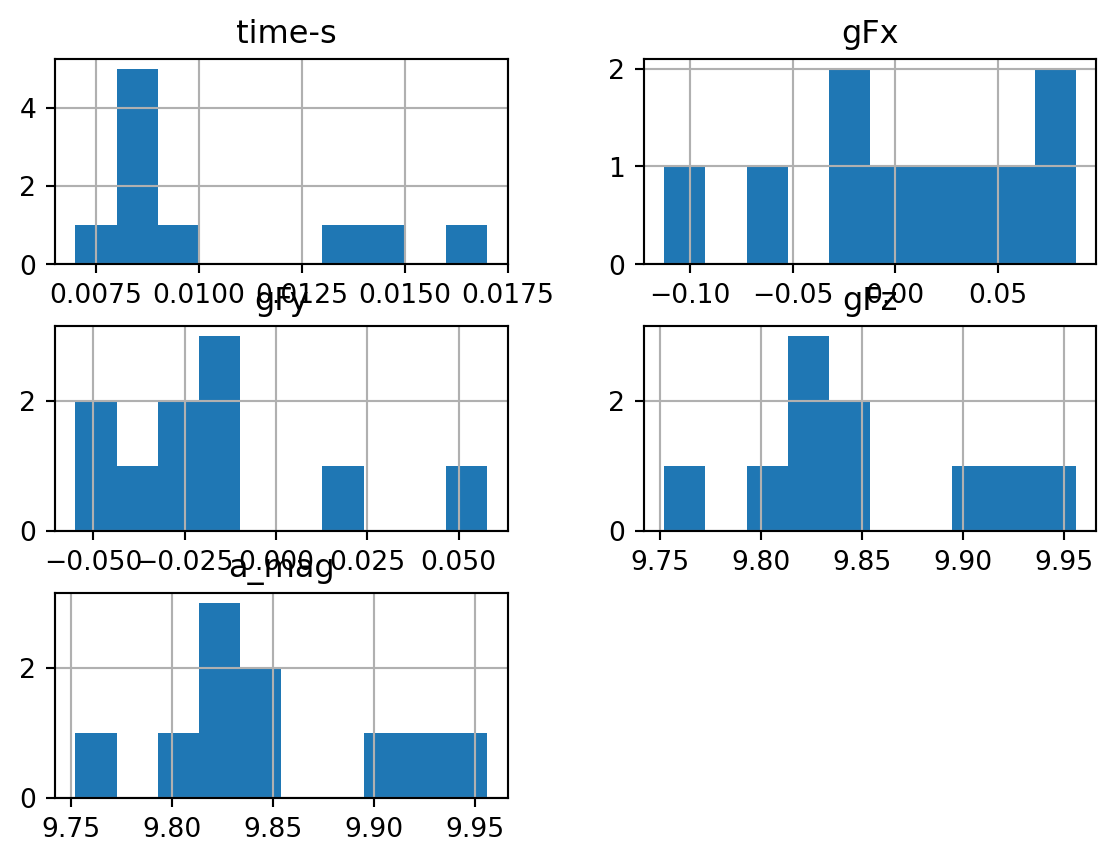
A histogram of each column can be easily generate with the dataframe.hist() function.
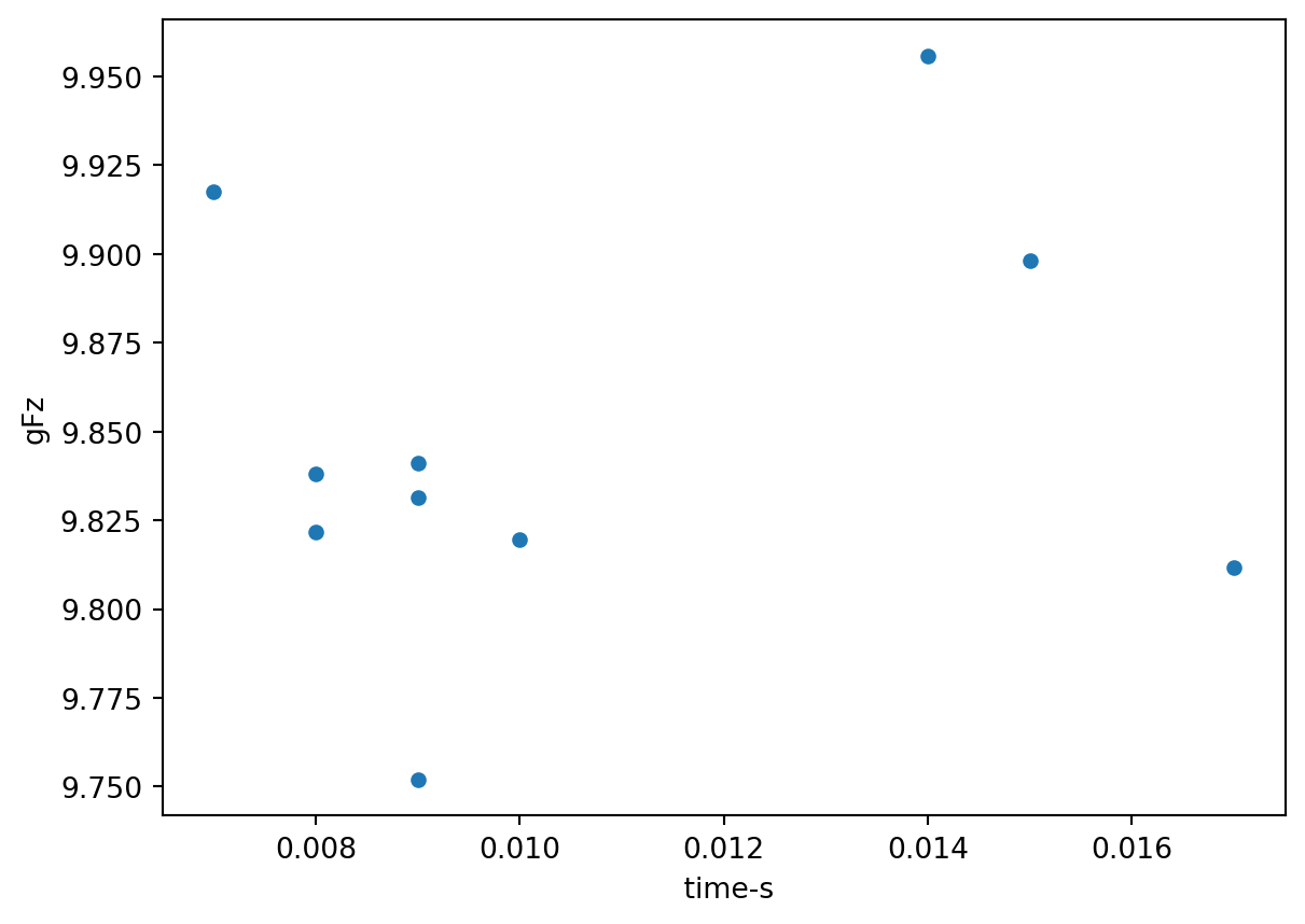
To make a scatter plot of two columns in your dataframe, use dataframe.plot.scatter(). The x and y keyword arguments should be used to specify which columns to plot.
elevator_data.plot.scatter(x =" time-s", y ="gFz")
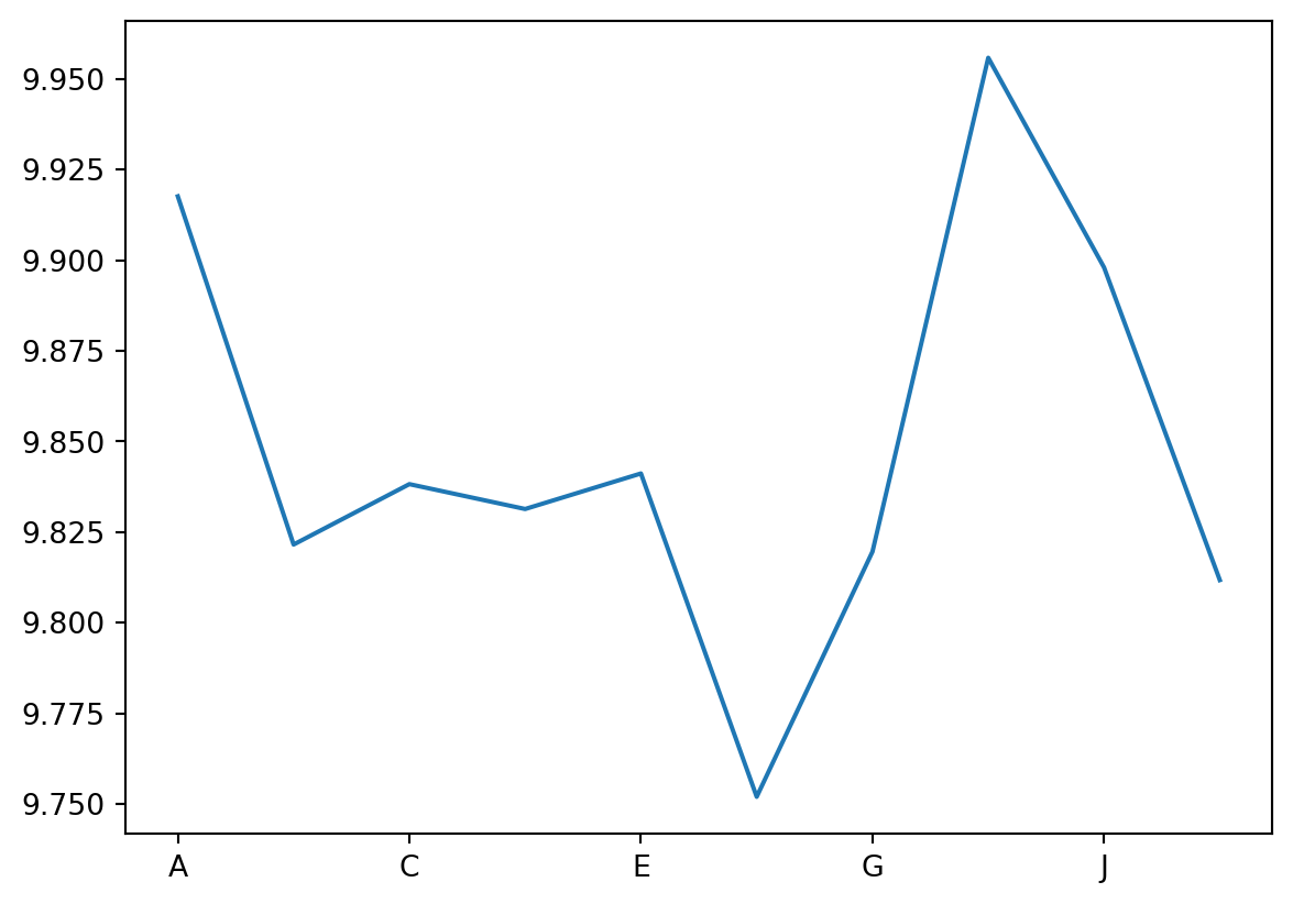
You can also plot a single column vs. the row labels using the plot function
elevator_data["gFz"].plot()
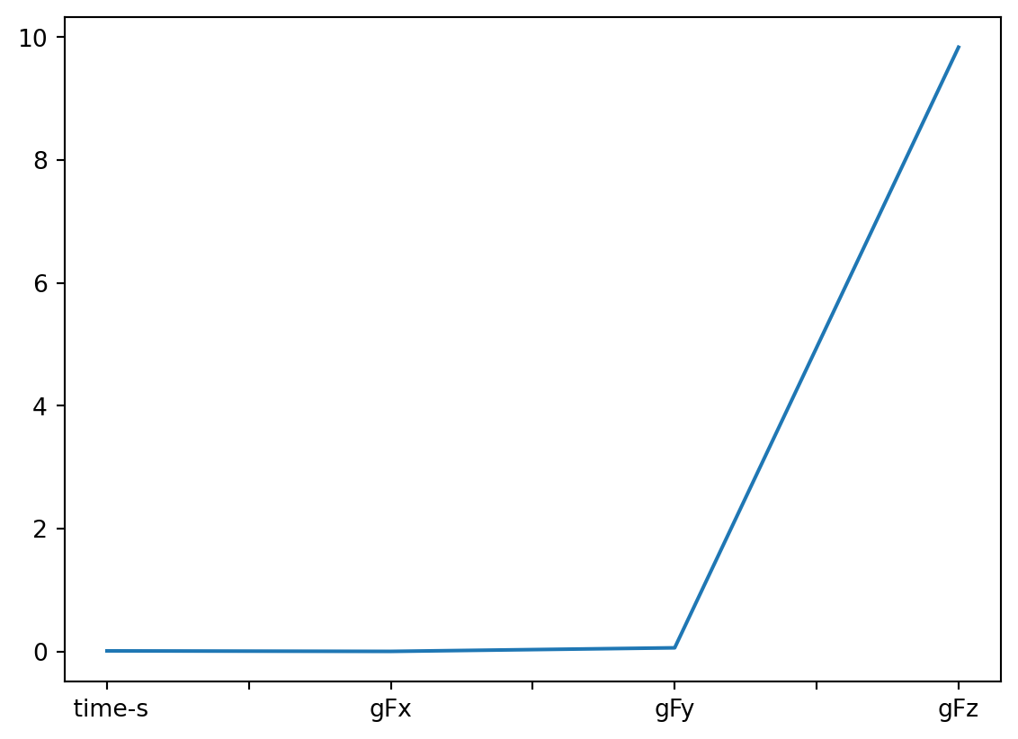
You can also use this function to plot a single row vs the column labels.
A wealth of other functions exist for pandas and I will not exemplify or explain them here because it is beyond the scope of the class. A nice summary sheet for pandas can be found here
13.5.3 Writing your dataframe to file
You have already used savetxt to save an entire array of numbers to a file in one step. If your data is in a pandas dataframe, saving that dataframe to file couldn’t be easier; just use dataframe.to_csv("filename").
elevator_data.to_csv("myelevatorData.csv")
Several helpful keyword arguments are available when writing to a file. I’ll list a few of them below.
sep - Delimiter or character used to separate the data as a length-one string. Default is a comma (“,”).
columns - specify which columns in your dataframe to write as a list of column labels.
index - True if you want the row labels written and False if you don’t
compression - specify the compression scheme as a string. Options are ‘zip’,‘gzip’, ‘bz2’,‘zstd’, and ‘tar’.
Depending on the type of data you are working with, there is a good argument for always using to_csv to write data to file, never needing savetxt.