Lab 2: Propagation of Uncertainty I
Name:
Skills
In this lab you will gain the following skills
- Construct Python dataframes and use them to display datasets.
- Construct arrays of plots in Python (multiple plots on one canvas).
- Use numpy arrays to perform mathematical calculations on data sets.
- Use \(\LaTeX\) to write simple math equations.
- Know the meaning of the derivative and partial derivative.
- Use derivatives to propagate uncertainty for moderately complex calculations.
Background Information
The Slope of a Function
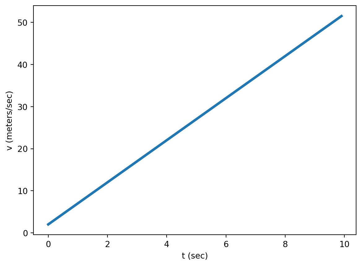
Mathematical functions describe how one quantity depends on one or more other quantities. For example, the velocity function
\[v(t) = 5 t + 2\]
gives the relationship between velocity and time.
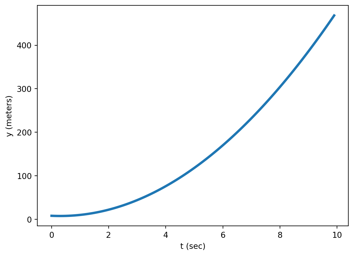
and this function gives the relationship between position and time
\[y(t) = 5t^2 -3t + 8\]
The slope of a function (\(m\)) is the rate at which the function changes with its variables. The slope is straightforward to calculate for linear functions: Just pick two points, calculate \(\Delta y = y_2 -y_1\) and \(\Delta t = t_2 - t_1\), and divide them. \[m = {\Delta y \over \Delta t}\]
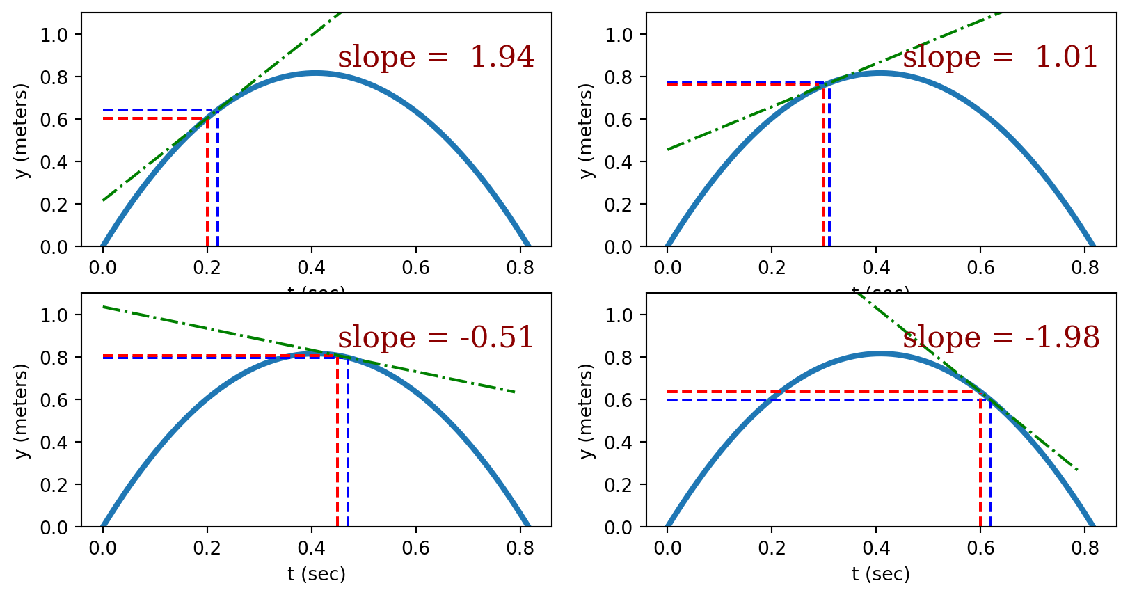
Generally, the slope of a function isn’t constant but varies across the domain. The figure below illustrates how the tangent line to a non-linear function varies across the domain.
For those that are interested, the slope of the tangent line of a function can be found by calculating the slope of a function in the limit that the change in \(x\) (\(\Delta x\)) becomes infinitely small.
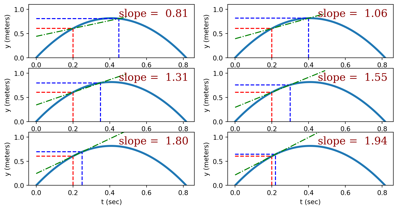
To reiterate: The slope isn’t a single number but rather another function. (The slope for linear functions is also a function, but since it’s a constant we sometimes forget this.) This sloping function can be evaluated at any point to determine the slope of the original function. For example, the slope of the function
\[y(t) = 4t - 4.9 t^2\]
is given by the sloping function
\[y'(t) = {dy(t) \over dt} = -9.8 t + 4\]
These functions are plotted below to illustrate their relationship.
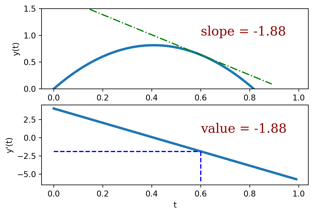
The notation \({dy(t) \over dt}\) is used to indicate the sloping function corresponding to \(y(t)\). (\(y'(t)\) is another common way to indicate this function.)
The derivative
The sloping function can be found by applying a set of mathematical rules to the function of interest. Most of the first half of calculus are devoted to the learning and mastery of these rules. One of the more common rules is the power rule which applies to polynomial functions. Specifically, if \(f(x) = a + bx + cx^2 + dx^2 + \dots = \sum_n a_n x^n\), then
\[ y(x) = f'(x) = a_n (n - 1) x^{n-1}\]
This rule was used to find the sloping function above. A plot of these two functions is given below.
To reiterate: the value of the sloping function (derivative) is equal to the slope of the original function. That’s a derivative.
The derivative of some other common functions is given in the table below. Your calculus class will teach you how to find the derivative of more complicated functions than those found in the table.
| Function (\(f(x)\)) | Derivative (\(y(x) = f'(x)\)) |
|---|---|
| \(f(x) = \sin(a x)\) | \(y(x) = a \cos(a x)\) |
| \(f(x) = \cos(a x)\) | \(y(x) = -a \sin(a x)\) |
| \(f(x) = \tan(a x)\) | \(y(x) = a \sec(a x)^2\) |
| \(f(x) = e^{a x}\) | \(y(x) = ae^{a x}\) |
| \(f(x) = \ln(a x)\) | \(y(x) = {a \over x}\) |
| \(f(x) = {a \over x}\) | \(y(x) = -{a \over x^2}\) |
Using the derivative to find uncertainty.
So how does the derivative help when calculating uncertainty. As a simple reminder: the slope of a function is the ratio of the change in function value to the change in variable value.
\[ \text{slope} = {\partial f \over \partial x} = {\text{rise} \over \text{run}} = {\delta f \over \delta x}\]
If \(\delta f\) is the uncertainty in a calculated value and \(\delta x\) is the uncertainty in the measured value, the equation above provides a way to calculate the uncertainty in the calculated value.
\[\delta f = \text{slope} \times \delta x = {\partial f \over \partial x}\]
Let’s consider an example where we measure the frequency (\(f\)) of a certain light beam to be \(f = 4.2 \pm 0.5 \times 10^{15}\) Hz and want to calculate the wavelength \(\lambda\) (with its associated uncertainty).
\[ \lambda(f) = {3 \times 10^8 \over f} = 7.14 \times 10^{-8}~ \text{m}\]
A plot of this function is given below
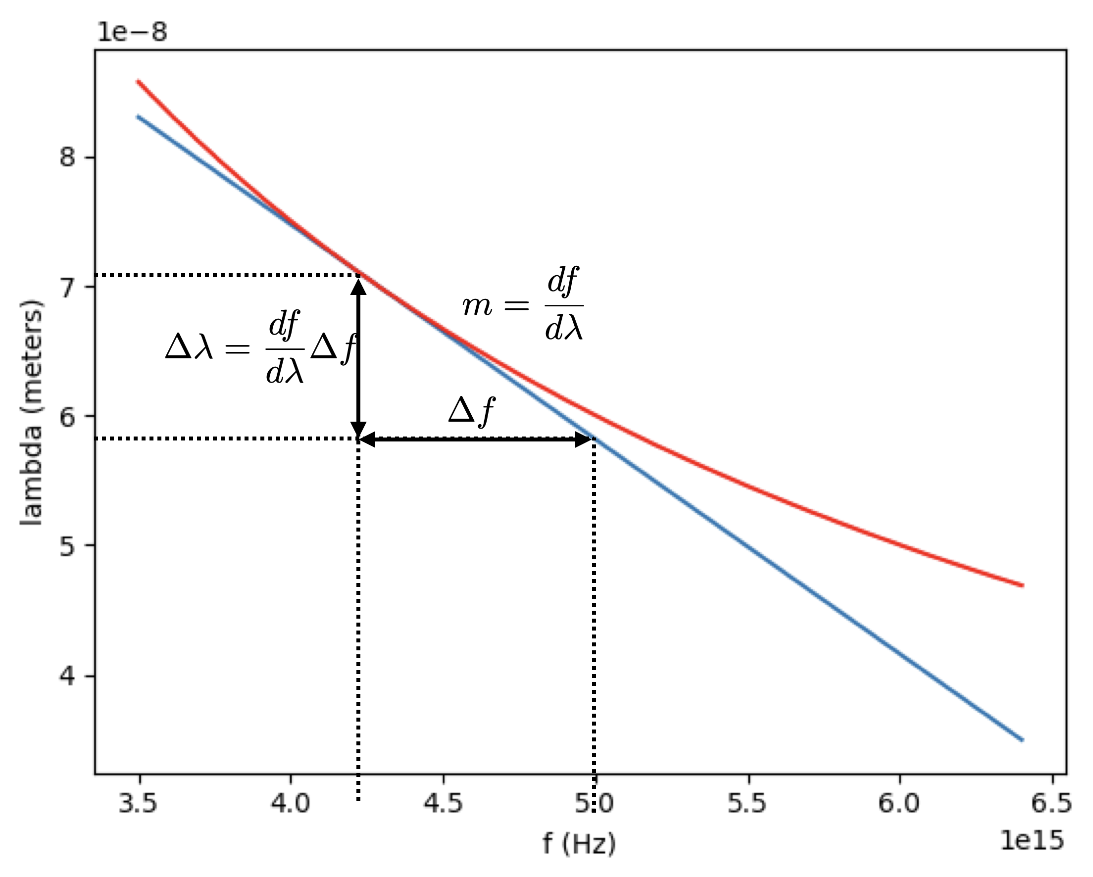
Using the table above to calculate the derivative we find
\[ \lambda'(f) = {\partial \lambda \over \partial f} = -{3 \times 10^8 \over f^2} \]
And hence, the unceratainty in the wavelength is:
\[\delta \lambda = {\partial \lambda \over \partial f} \delta f \] \[ = -{3 \times 10^8 \over f^2} \delta f\] \[= -{3 \times 10^8 \over (4.25 \times 10^{15} ~\text{Hz})^2} (0.5 \times 10^{15} ~\text{Hz})\] \[ = 8.5 \times 10^9 ~ \text{m}\]
Partial Derivatives
When the function of interest has more than one independent variable, derivatives are performed on each variable separately, and all other variables are treated as constants. Derivatives of functions of many variables are called partial derivatives.
For example, consider the function:
\[f(x,y) = 5 x y^2 + 8 x^2 y\]
The partial derivatives of this function are
\[{\partial f \over \partial x} = 5 y^2 + 16 x y\] \[{\partial f \over \partial y} = 10 xy + 8 x^2\]
The uncertainty in the calculated values is calculated by first forming the product \({\partial f \over \partial x_i} \delta x_i\) for each independent variables and inserted into the equation below \[(\delta f)^2 = ({\partial f\over \partial x} \delta x)^2 + ({\partial f\over \partial y}\delta y)^2 + \dots\]
This is the most important formula for uncertainty propagation and the one we will use going forward.
An Example
Imagine measuring the dimensions and mass of a block with their associated uncertainties:
\[l = 5.2 \pm 0.1 ~\text{cm}\] \[w = 8.4 \pm 0.3 ~\text{cm}\] \[h = 10.8 \pm 0.4 ~\text{cm}\] \[m = 345 \pm 5 ~\text{grams}\]
and proceeding to calculate the density of the block
\[\rho = {m \over V} = {m \over l \times w \times h}\]
= 0.73 g/cm^3To calculate the uncertainty, we must first take four derivatives with respect to \(l\), \(w\), \(h\), and \(m\):
\[ {\partial \rho \over \partial l} = -{m \over l^2 w h}\]
\[ {\partial \rho \over \partial h} = -{m \over l w h^2}\]
\[ {\partial \rho \over \partial w} = -{m \over l w^2 h}\]
\[ {\partial \rho \over \partial m} = {1 \over l w h}\]
Now we can calculate the uncertainty as
\[\delta \rho = \sqrt{({\partial \rho \over \partial l} \delta l)^2 + ({\partial \rho \over \partial w} \delta w)^2 + ({\partial \rho \over \partial h} \delta h)^2 + ({\partial \rho \over \partial m} \delta m)^2}\]
\[ = \sqrt{(-{m \over l^2 w h} \delta l)^2 + (-{m \over l w^2 h} \delta w)^2 + (-{m \over l w h^2} \delta h)^2 + ({1 \over l w h} \delta m)^2}\]
\[ = \sqrt{(-{(345 ~\text{grams}) \over (5.42 ~\text{cm})^2 (8.4 ~\text{cm}) (10.8 ~\text{cm})} (0.1 ~\text{cm}))^2 + (-{(345 ~\text{grams}) \over (5.42 ~\text{cm}) (8.4 ~\text{cm})^2 (10.8 ~\text{cm})} (0.3 ~\text{cm}))^2 + (-{(345 ~\text{grams}) \over (5.42 ~\text{cm}) (8.4 ~\text{cm}) (10.8 ~\text{cm})^2} (0.4 ~\text{cm}))^2 + ({1 \over (5.42 ~\text{cm}) (8.4 ~\text{cm}) (10.8 ~\text{cm})} (5 ~\text{grams}))^2}\]
In the code cell below we use python to calculate this uncertainty. Note that we use a formatted print statement to display the uncertainty to one significant figure.
from numpy import sqrt
m = 345
dm = 5
l = 5.2
dl = 0.1
w = 8.4
dw = 0.3
h = 10.8
dh = 0.4

rho = m/l/w/h
drdl = -m/l**2/w/h
drdw = -m/l/w**2/h
drdh = -m/l/w/h**2
drdm = 1/l/w/h
drho = sqrt((drdl * dl)**2 + (drdw * dw)**2 + (drdh * dh)**2 + (drdm * dm)**2)
print(f"The density of the block is {rho:5.2f} +- {drho:4.2f} g/cm^3")
The density of the block is 0.73 +- 0.04 g/cm^3Python Skills
DataFrames
A dataframe is a data structure that organizes data into a 2-dimensional table of rows and columns, similar to a spreadsheet. A dataframe can be initiated in Python using the pandas.DataFrame() function (case sensitive). For example, suppose that you used the accelerometer on your phone to gather the following data.
   time     gFx     gFy     gFz
0  0.007 -0.0056 -0.0046  1.0120
1  0.008  0.0007  0.0024  1.0022
2  0.008  0.0000  0.0059  1.0039
3  0.009  0.0054 -0.0022  1.0032
4  0.009 -0.0015 -0.0056  1.0042
5  0.009  0.0037 -0.0020  0.9951
6  0.010 -0.0020 -0.0020  1.0020
7  0.014  0.0090 -0.0024  1.0159
8  0.015  0.0012 -0.0037  1.0100
9  0.017 -0.0115 -0.0020  1.0012
This data can be loaded into a dataframe like this.
from pandas import DataFrame
import numpy as np

time = [0.007,0.008,0.008,0.009,0.009,0.009,0.01,0.014,0.015,0.017]
gFx = [-0.0056,0.007,0,0.0054,-0.0015,0.0037,-0.002,0.009,0.0012,-0.0115]
gFy = [-0.0046,0.0024,0.0059,-0.0022,-0.0056,-0.002,-0.002,-0.0025,-0.0037,-0.002]
gFz = [1.012,1.0022,1.0039,1.0032,1.0042,0.9951,1.002,1.0159,1.01,1.0012]
elevator_data = DataFrame(np.transpose([time,gFx,gFy,gFz]),columns = ["time", "gFx","gFy", "gFz"])
display(elevator_data)| time | gFx | gFy | gFz | |
|---|---|---|---|---|
| 0 | 0.007 | -0.0056 | -0.0046 | 1.0120 |
| 1 | 0.008 | 0.0070 | 0.0024 | 1.0022 |
| 2 | 0.008 | 0.0000 | 0.0059 | 1.0039 |
| 3 | 0.009 | 0.0054 | -0.0022 | 1.0032 |
| 4 | 0.009 | -0.0015 | -0.0056 | 1.0042 |
| 5 | 0.009 | 0.0037 | -0.0020 | 0.9951 |
| 6 | 0.010 | -0.0020 | -0.0020 | 1.0020 |
| 7 | 0.014 | 0.0090 | -0.0025 | 1.0159 |
| 8 | 0.015 | 0.0012 | -0.0037 | 1.0100 |
| 9 | 0.017 | -0.0115 | -0.0020 | 1.0012 |
The display command can then be used to display the dataframe to screen. The keyword argument columns = ["time", "gFx","gFy", "gFz"] will assign names to the columns of the dataframe. The rows also have names attached but since these names were not specified, they defaulted to the integers 0 - 9. If you want to assign different names to the rows of your dataframe, add the keyword argument index = when you call DataFrame, like this
from pandas import DataFrame
import numpy as np

time = [0.007,0.008,0.008,0.009,0.009,0.009,0.01,0.014,0.015,0.017]
gFx = [-0.0056,0.007,0,0.0054,-0.0015,0.0037,-0.002,0.009,0.0012,-0.0115]
gFy = [-0.0046,0.0024,0.0059,-0.0022,-0.0056,-0.002,-0.002,-0.0025,-0.0037,-0.002]
gFz = [1.012,1.0022,1.0039,1.0032,1.0042,0.9951,1.002,1.0159,1.01,1.0012]
elevator_data = DataFrame(np.transpose([time,gFx,gFy,gFz]),columns = ["time", "gFx","gFy", "gFz"],index = ["A","B","C","D","E","F","G","H","J","K"])
display(elevator_data)| time | gFx | gFy | gFz | |
|---|---|---|---|---|
| A | 0.007 | -0.0056 | -0.0046 | 1.0120 |
| B | 0.008 | 0.0070 | 0.0024 | 1.0022 |
| C | 0.008 | 0.0000 | 0.0059 | 1.0039 |
| D | 0.009 | 0.0054 | -0.0022 | 1.0032 |
| E | 0.009 | -0.0015 | -0.0056 | 1.0042 |
| F | 0.009 | 0.0037 | -0.0020 | 0.9951 |
| G | 0.010 | -0.0020 | -0.0020 | 1.0020 |
| H | 0.014 | 0.0090 | -0.0025 | 1.0159 |
| J | 0.015 | 0.0012 | -0.0037 | 1.0100 |
| K | 0.017 | -0.0115 | -0.0020 | 1.0012 |
Now the names of your rows will be “A” through “K”
Multiple Plots
Last week we learned how to generate a single, simple plot. Often you may want to generate multiple, independent plots in the same figure. To do this, first we must use the figure function which generates the canvas upon which the plots will appear. Assign this object to a variable so you can refer to it later. To create each subplot, the fig.add_subplot(rows,columns, plot_number) function is used. There are three arguments to this function; the first two indicate the shape of the grid and the third indicates which position on the grid this plot will be assigned.
fig.add_subplot(rows,columns,plot_location)After the axes object has been created, we can call the plot, or errorbar function again, and a plot will be generated at its location. Here is an example that will generate two plots side by side.
from matplotlib import pyplot as plt
%matplotlib inline
from numpy import linspace,sqrt

r = linspace(0.9,4,50)

sigmaOne = 1
epsilonOne = 1
sigmaTwo = 2
epsilonTwo = 2
energyOne = 4 * sigmaOne* ((epsilonOne/r)**12 - (epsilonOne/r)**6)
energyTwo = 4 * sigmaTwo * ((epsilonTwo/r)**12 - (epsilonTwo/r)**6)

fig = plt.figure()
ax1 = fig.add_subplot(1,2,1)
ax2 = fig.add_subplot(1,2,2)

ax1.plot(r,energyOne,marker = '+',color = 'k')
ax1.set_xlim(0.5,3.0)
ax1.set_ylim(-1.5,5)
ax1.set_xlabel("Separation Distance")
ax1.set_ylabel("Energy")
ax1.set_title("Lennard-Jones Potential")

ax2.plot(r,energyTwo,marker = 'o',color = 'r')
ax2.set_xlim(0.5,4.0)
ax2.set_ylim(-2,5)
ax2.set_xlabel("Separation Distance")
ax2.set_ylabel("Energy")
ax2.set_title("Lennard-Jones Potential")
Text(0.5, 1.0, 'Lennard-Jones Potential')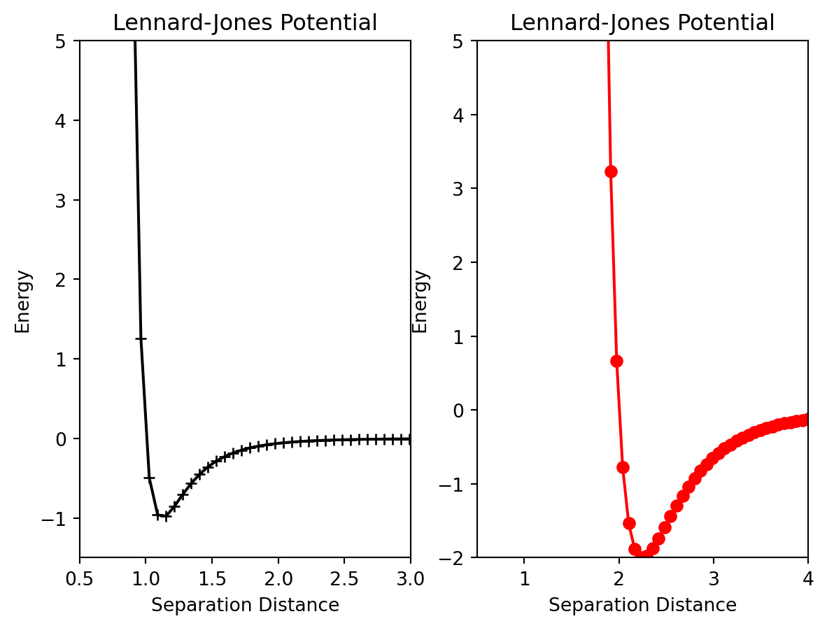
Pay close attention to the add_subplot function. ax1=add_subplot(1,2,1) will generate a \(1\) x \(2\) grid of plots and ax1 will correspond plot at the 1st location. Below is an example of a more advanced array of plots. Pay close attention to the add_subplot functions until you understand.
from matplotlib import pyplot as plt
%matplotlib inline
from numpy import linspace,sqrt

r = linspace(0.9,4,50)

sigmaOne = 1
epsilonOne = 1
sigmaTwo = 2
epsilonTwo = 2
energyOne = 4 * sigmaOne* ((epsilonOne/r)**12 - (epsilonOne/r)**6)
energyTwo = 4 * sigmaTwo * ((epsilonTwo/r)**12 - (epsilonTwo/r)**6)

fig = plt.figure()
ax1 = fig.add_subplot(2,1,1)
ax2= fig.add_subplot(2,2,3)
ax3 = fig.add_subplot(2,2,4)

ax1.plot(r,energyOne,marker = '+',color = 'k')
ax1.set_xlim(0.5,3.0)
ax1.set_ylim(-1.5,5)
ax1.set_xlabel("Separation Distance")
ax1.set_ylabel("Energy")
ax1.set_title("Lennard-Jones Potential")

ax2.plot(r,energyTwo,marker = 'o',color = 'r')
ax2.set_xlim(0.5,4.0)
ax2.set_ylim(-2,5)
ax2.set_xlabel("Separation Distance")
ax2.set_ylabel("Energy")
ax2.set_title("Lennard-Jones Potential")

ax3.plot(r,energyTwo,marker = 'o',color = 'r')
ax3.set_xlim(0.5,4.0)
ax3.set_ylim(-2,5)
ax3.set_xlabel("Separation Distance")
ax3.set_ylabel("Energy")
ax3.set_title("Lennard-Jones Potential")
plt.tight_layout()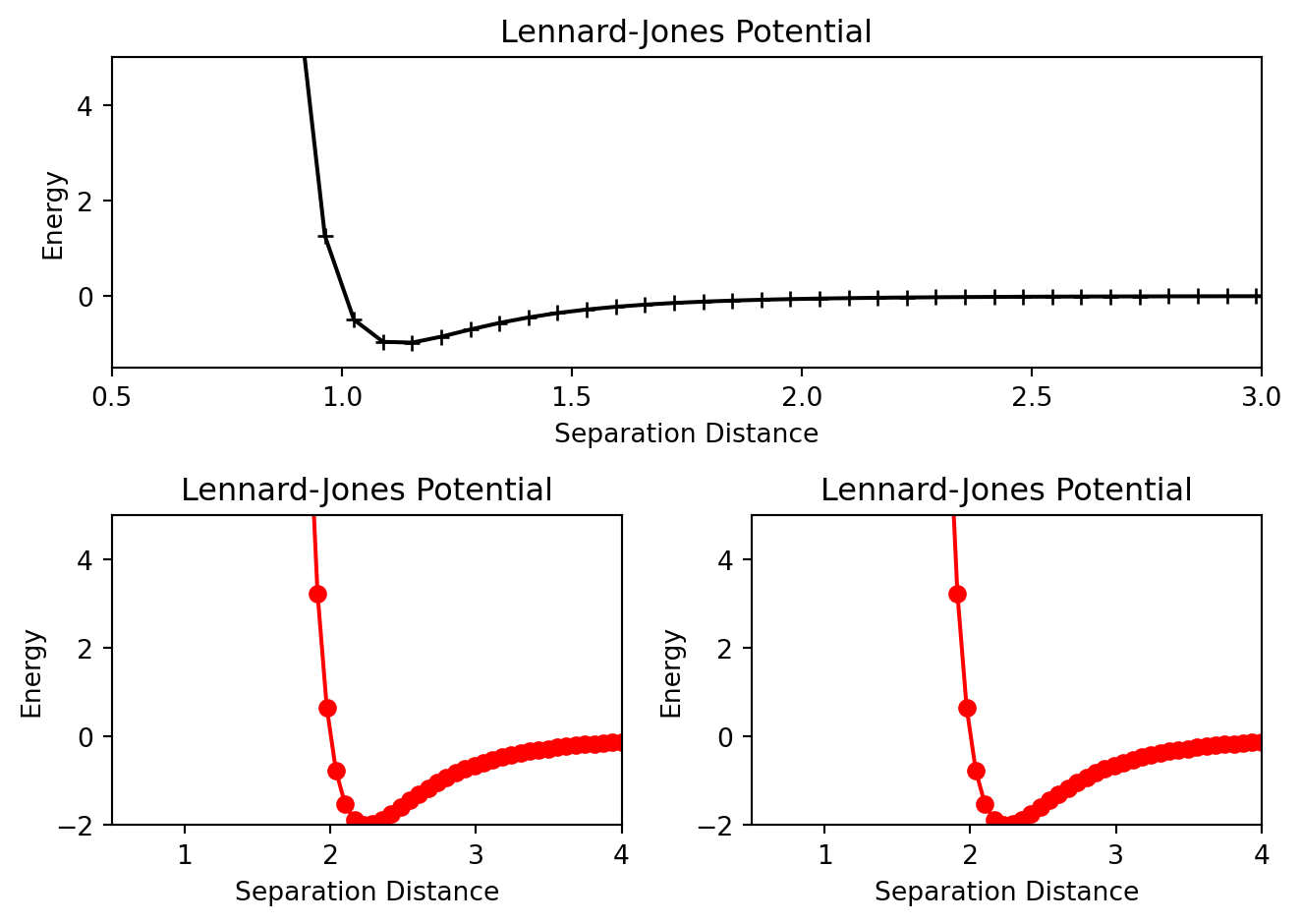
Also notice the set_xlim, set_ylim, set_xlabel etc methods that were used to customize each individual plot. There are a host of other methods available for further customization.
This website has a comprehensive list of them.
Numpy Arrays
Often in science you’ll be working with more than one data point at a time. For example, consider the data shown below of a ball that is dropped from several different initial heights.
| Initial height (meters) | Fall time (seconds) | |
|---|---|---|
| 0 | 2.0 | 0.64 |
| 1 | 2.5 | 0.71 |
| 2 | 3.0 | 0.78 |
| 3 | 3.5 | 0.85 |
| 4 | 4.0 | 0.90 |
Data like this should be stored in a numpy (“num-pie”) array, like this:
import numpy as np

t = np.array([0.64,0.71,0.78,0.85,0.90])
y = np.array([2.0,2.5,3.0,3.5,4.0])
The benefit of storing your data in arrays is that mathematical calculations are “vectorized” which means that the mathematical operation is performed across the entire data set without needing a loop. For example, the equation \(g = {2 y \over t^2}\) could be used to find the acceleration due to gravity for all of the data points like this:
import numpy as np

t = np.array([0.64,0.71,0.78,0.85,0.90])
y = np.array([2.0,2.5,3.0,3.5,4.0])

g = 2 * y/t**2
print(g)
[9.765625 9.91866693 9.86193294 9.68858131 9.87654321]If you need to use mathematical function like square roots or trigonometric functions, you should always import them from numpy and not math.
\(\mathrm{\LaTeX}\)
Often you will want to include math equations as part of your explanation/text. Below is an example of what your math should and should not look like.
- \(|\vec{v}| = \sqrt{v_x^2 + v_y^2}\) (like this)
- v = sqrt(vx^2 + vy^2) (not like this)
To make your math equations look like the first example, you must enclose your math equation in “$$”, one pair at the beginnning of the equation and one pair at the end. Enclosing your expression in double dollar signs will put the expression on its own line. To place the expression in the middle of a sentence (inline) you’ll need to enclose the expression in single dollar signs. To generate the math symbols that often show up in equations, you’ll need to know the correct syntax. A table of commonly used math symbols is given below.
| Math symbol | Example | \(\mathrm{\LaTeX}\) syntax |
|---|---|---|
| Subscript | \(v_x\) | v_x |
| Powers | \(v^2\) | v^2 |
| Powers with more than one digit | \(v^{10}\) | v^{10} |
| Square root | \(\sqrt{a + b}\) | \sqrt{a + b} |
| Fractions | \(\frac{a}{b}\) | \frac{a}{b} |
| Vectors | \(\vec{x}\) | \vec{x} |
| Integrals | \(\int x^2 dx\) | \int x^2 dx |
| Partial Derivatives | \({\partial f \over \partial x}\) | {\partial f \over \partial x} |
| Summations | \(\sum_{i = 1}^{10} x_i^2\) | \sum_{i = 1}^{10} x_i^2 |
| Infinity | \(\infty\) | \infty |
You can include Greek letters in your expressions if you know the corresponding syntax. The table below shows some of the more common Greek letters used in physics.
| Greek Letter | \(\mathrm{\LaTeX}\) syntax |
|---|---|
| \(\alpha\) | \alpha |
| \(\beta\) | \beta |
| \(\gamma\) | \gamma |
| \(\Delta\) | \Delta |
| \(\epsilon\) | \epsilon |
A more comprehensive list of math symbols available can be found here
Activity I: The pendulum (50 pts)
Equipment needed:
- Pendulum. (We have some pre-made, or you can tie a string to a mass)
- Metal support stand for pendulum to swing from.
- Photogate.
Goal:
By taking measurements on a simple pendulum, calculate the acceleration due to gravity with its associated uncertainty. Compare to the known value for Rexburg.
Procedure:
- Assemble five pendulums of different lengths, with the lengths ranging from \(0.25\) m to \(2.0\) m.
- For each pendulum, perform the following:
- Measure the distance from the support point to the center of the pendulum. This is the length of the pendulum \(L\). Assign an uncertainty to this measurement.
- Release the pendulum from a small initial angle (no bigger than \(15^\circ\) from the vertical) and use the photogate to measure the period \(T\) of the pendulum with its associated uncertainty. (The period of a pendulum is the time it take to make one full cycle.)
- Place all of your lengths and periods and their uncertainties into numpy arrays.
- Calculate the acceleration due to gravity (\(g\)) using \(g = {4 \pi^2 L \over T^2}\).
- Using the methods discussed above determine the equation for calculating the uncertainty in \(g\). Use \(\LaTeX\) syntax to complete the math equation below \[ \delta g = \]
- Calculate the uncertainty and fractional uncertainty in \(g\) in the code cell below.
- Put your data in a dataframe and display the dataframe to visually verify that it has 10 rows and 6 columns. The columns should be \(L\), \(T\), \(g\) and their uncertainties. Give the appropriate names.
- Construct a multi-figure plot containing two plots. The first plot should be period vs length and the other plot should be g vs. length. The points on both plots should have error bars attached.
- Add axes labels and titles to both of your plots.
- Analyze the results to answer the following questions:
- Which result has the lowest uncertainty? Can you explain why?
- What function do you think best represents the relationship between \(L\) and \(T\)?(We will study curve-fitting in a later lab.)
- The accepted value of \(g\) for Rexburg is \(g = 9.80056\) m/s\(^2\). Do your calculations agree with this value to within your calculated uncertainties?
Response:
import matplotlib.pyplot as plt
import pandas as pd
import numpy as np
%matplotlib inline


T =    # Create array of period values.
un_T =  # Create array of uncertainties in the period measurements.
L =     # Create array of length values.
un_L =  # Create array of uncertainties in the length measurements.
g =     # Calculate g for the whole data set.
un_g =   # Calculate the uncertainty in g for the whole data set.
frac_un =  # Calculate fractional uncertainties.

df =            # Creat a dataframe of your data. Give the columns appropriate names
display(df) # Display the dataframe

# Construct a multi-figure plot below.
fig = plt.figure()

plt.show()
Activity II (50 points)
Equipment needed
- Meter Stick
- Stopwatch (the one on your phone will do fine.)
- Tennis ball.
Goal
By measuring the fall time for an object in free fall, calculate the acceleration due to gravity here in Rexburg. You’ll be dropping a tennis ball from 10 different heights and measuring the fall time for each.
Procedure
- Find a location in the building that will allow the greatest drop distance for the tennis ball. (The front foyer is a good choice.) You’ll be dropping the tennis ball from 10 different heights starting at \(1\) meter and ending at the largest height you can achieve. Measure the height.
- Using a stopwatch, measure the fall time with its associated uncertainty. Record the values in the code cell provided below. Note: typical reaction times are around \(0.25\) s.
- Repeat steps 1 and 2 ten more times to obtain ten data points. The ball should be dropped from a different height for each trial. Place your heights and drop times and their uncertainties in numpy arrays.
- Using the equation below, calculate the acceleration due to gravity for all 10 data points. \[ g = {2 h \over t^2}\]
- Using the methods discussed above determine the equation for calculating the uncertainty in \(g\). Use \(\LaTeX\) syntax to complete the math equation below \[ \delta g = \]
- Using the equation from step 5, calculate the uncertainty in \(g\) in the code cell below for all 10 data points.
- Put your data in a dataframe and display the dataframe to visually verify that it has 10 rows and 6 columns.
- Construct a multi-figure plot containing two plots. The first plot should be \(g\) vs trial number and the other plot should be \(g\) vs. fall time. The points on both plots should have error bars attached.
- Add axes labels and titles to both of your plots.
- Using your results, answer the following questions:
- Are your ten g values consistent with one another to within their stated uncertainties. Explain.
- What function do you think describes the relationship between the fall distance and the fall time. (We will study curve-fitting in a later lab.)
- Which of your g values agree with the accepted value of g for Rexburg given in the first exercise.
Response:
import matplotlib.pyplot as plt
import numpy as np
import pandas as pd
%matplotlib inline

trial = np.array([1,2,3,4,5,6,7,8,9,10])
h =   # Construct an array of the fall distances
un_h =     # Construct an array of the uncertainties in the fall distances.
t =       # Construct an array of the measured fall times.
un_t =        # Construct an array of the uncertainties in the fall times.
g =               # Calculate g for the entire data set.
un_g =            # Calculate the uncertainty in g
frac_g =          # Calculate the fractional uncertainty.

df = # Create a dataframe of your data. Give the columns appropriate names
display(df) # Display your dataframe


# Construct plots
fig = plt.figure()


plt.show()