Text(0.5, 1.0, 'Skid time vs initial speed')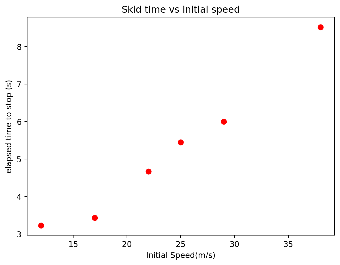
Name:
Often in science you will gather data as a way to explore the relationship between two physical quantities and/or to validate your theories. For example, consider the time it takes a car to stop, starting from the moment you slam on your brakes(locking them in place and skidding to a halt). The question is: How does the stopping time depend on the car’s initial speed. If you are familiar with Newtonian mechanics at all, you might hypothesize that the acceleration of the car should not depend on the initial velocity and hence the stopping time will increase linearly with the initial speed. Furthermore, the following kinematic equation
\[
\begin{align*}
v_f &= v_i - a \Delta t\\
0 &= v_i - \mu_k g \Delta t\\
\Delta t &= {v_i\over \mu_k g}
\end{align*}
\] would suggest that the slope of \(\Delta t\) vs. \(v_i\) function is \({1\over a} = {1\over \mu g}\). In other words, the theory of kinematics suggest that the acceleration should be independent of initial speed. To prove your idea, you should first measure the stopping time for cars with a variety of initial speeds (shown below).
| Initial Speed (m/s) | Skid time (s) |
|---|---|
| 12 | 3.23 |
| 17 | 3.43 |
| 22 | 4.67 |
| 25 | 5.45 |
| 29 | 6.00 |
| 38 | 8.52 |
Text(0.5, 1.0, 'Skid time vs initial speed')
We notice that the data looks linear which matches our hypothesis that the acceleration is constant.
The next thing to do is to find the line that passes through the data points as close as possible. When the fit function is a polynomial , we can use the polyfit function from numpy. This function takes three argument: the independent data set, the dependent data set, and the order of the polynomial
polyfit(x,y,order)The polyfit function returns a list of numbers containing the function parameters for the best fit function.
from matplotlib import pyplot as plt
from numpy import polyfit

t = [3.23,3.43,4.67,5.45,6,8.52]
vi = [12,17,22,25,29,38]

params = polyfit(vi,t,1)
slope = params[0]
yint = params[1]

g=9.8 #Acceleration due to gravity
mu = 1/(slope * g)
print(params)
print(mu)
[0.20971747 0.21840032]
0.48656326406696404In this case, \(0.2097\) is the slope of the best-fit function and \(0.2184\) is the y-intercept of the best fit function. Remembering our theory from above, we notice that the slope of this fit function can be used to calculate the coefficient of friction between the rubber tires and the roadway. \[ \begin{align*} m &= {1\over \mu g}\\ \mu &= {1\over m g} \end{align*} \] It is often useful to plot the fit function on top of the data to verify that it really matches the data.
from matplotlib import pyplot as plt
from numpy import polyfit,linspace

t = [3.23,3.43,4.67,5.45,6,8.52]
vi = [12,17,22,25,29,38]

params = polyfit(vi,t,1)
vDense = linspace(8,40,100)
tDense = params[0] * vDense + params[1]

plt.plot(vi,t,'r.',ms = 16)
plt.plot(vDense,tDense,'k',lw = 3)
plt.xlabel("Initial Speed(m/s)")
plt.ylabel("elapsed time to stop (s)")
plt.title("Skid time vs initial speed")
Text(0.5, 1.0, 'Skid time vs initial speed')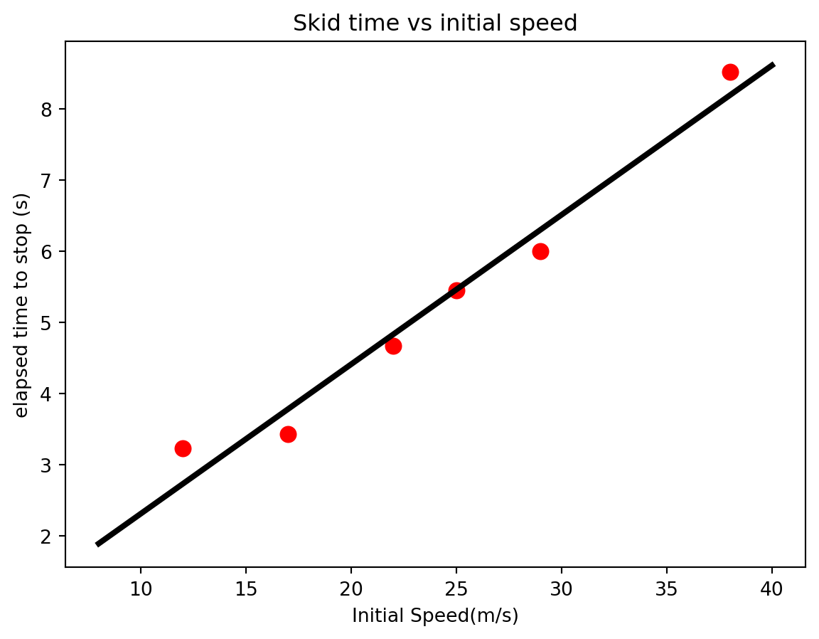
The uncertainty in the fit parameters can be determined by polyfit by adding the optional argument cov=True when you call it. This causes the polyfit function to return two things: 1- a list of parameter values (the slope and y-intercept for our case) and 2- a matrix of covariance values, the diagonal value of which are the standard deviations squared. Let’s see how we could access these numbers and display them.
from matplotlib import pyplot as plt
import numpy as np

t = [3.23,3.43,4.67,5.45,6,8.52]
vi = [12,17,22,25,29,38]

params = np.polyfit(vi,t,1,cov = True)
slope = params[0][0]
dslope = np.sqrt(params[1][0][0])
yint = params[0][1]
dyint = np.sqrt(params[1][1][1])

print(f"The slope is {slope:5.2f} +- {dslope:2.2f}")
print(f"The y-int is {yint:5.2f} +- {dyint:2.2f}")
The slope is 0.21 +- 0.02
The y-int is 0.22 +- 0.48The data above was linear, just like our hypothesis suggested, but this won’t be the case for many realistic data sets. One “tool” that a scientist frequently uses to investigate possible relationship is to attempt to linearize the data using a hypothesis. As an example, consider dropping a ball from rest, and measuring how far it has fallen at regular time intervals. Kinematics tells us that the relationship between \(y\) (the distance fallen) and \(t\) (the time elapsed) is: \[y = {1\over 2} g t^2\] where \(g\) is the acceleration due to gravity. This equation represents our hypothesis, which means that we don’t expect the relationship between \(y\) and \(t\) to be linear. The plot of \(y\) vs. \(t\) looks like this:
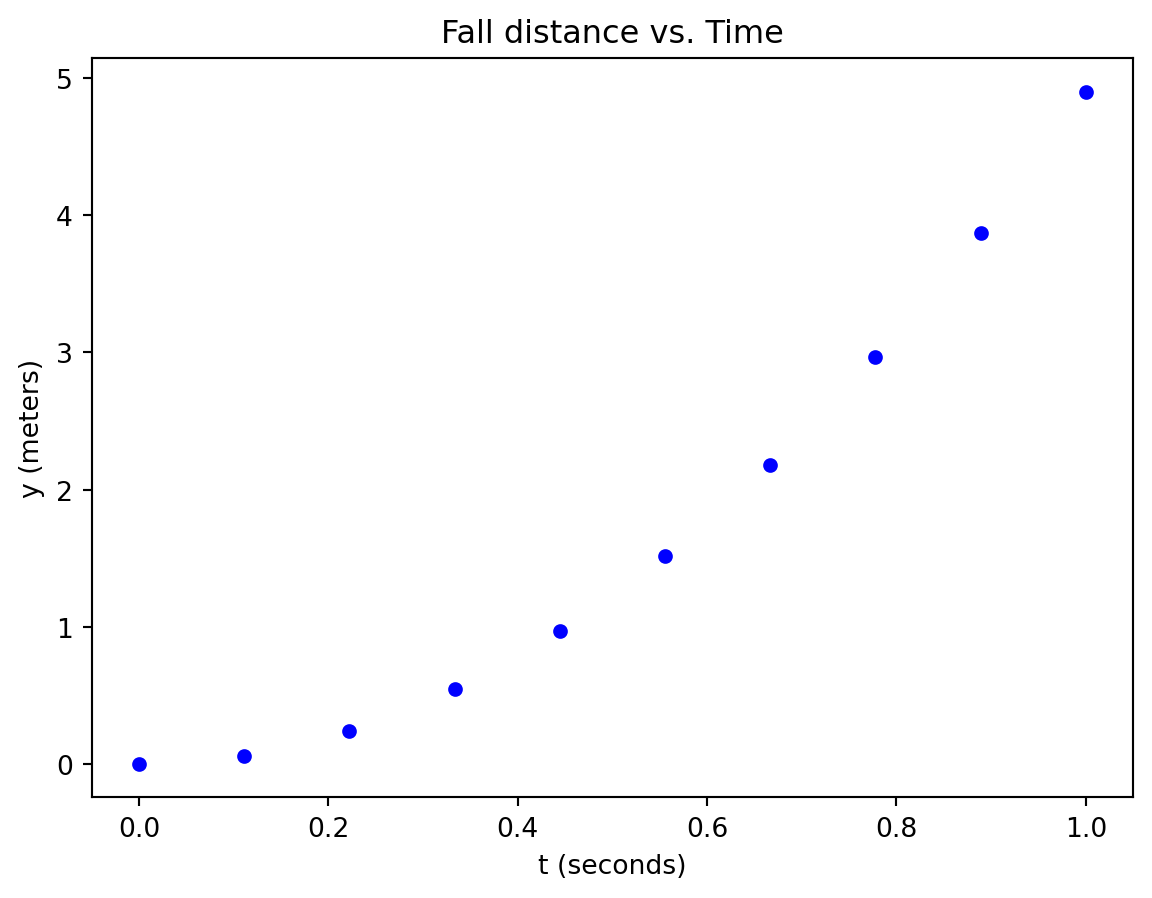
That is definitely not a linear relationship. But the data can be manipulated to become linear by following these steps:
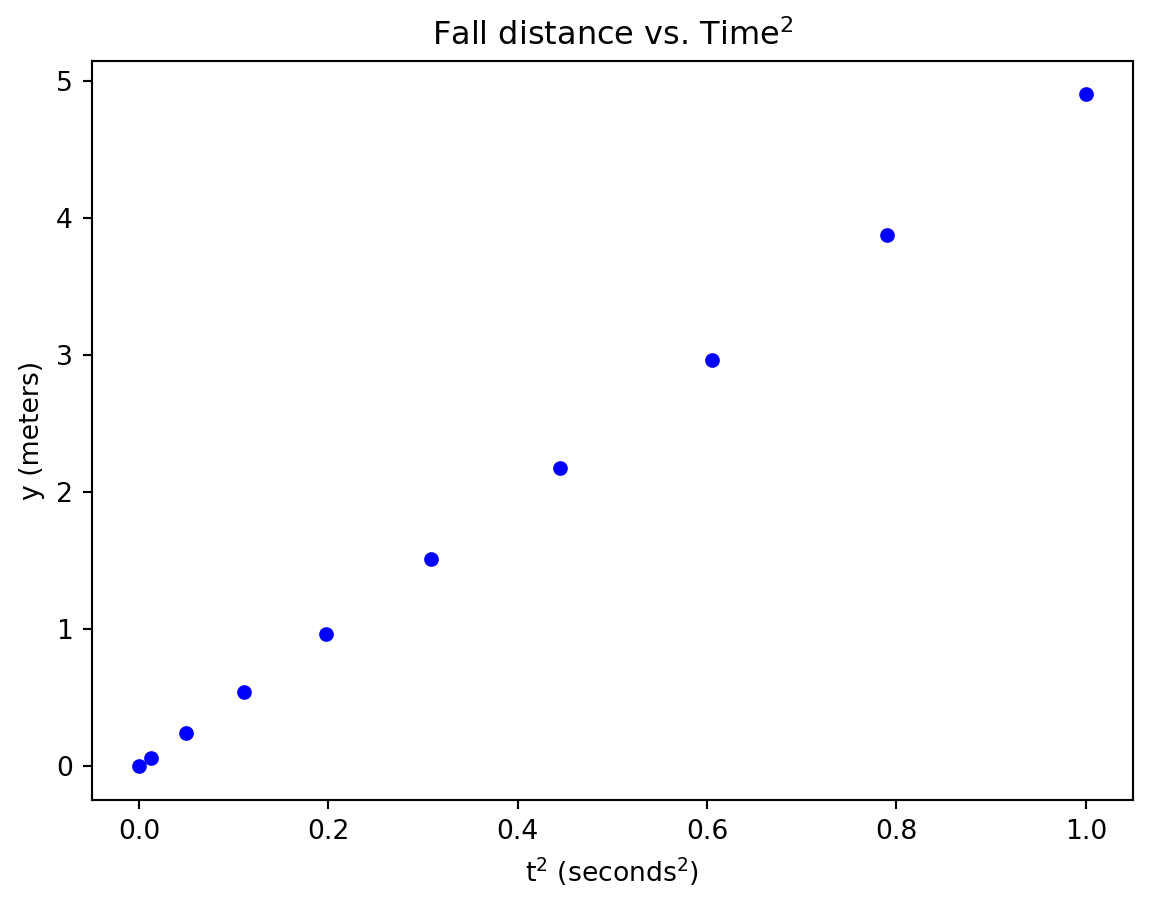
and indeed it does.
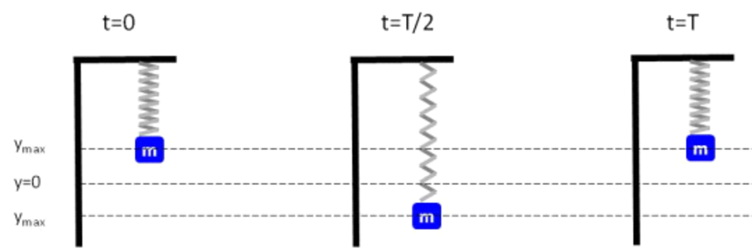
One of the objectives of this course is to learn how to design and carry out a successful experiment. In grade-school an experiment was any science related activity (the proverbial building of a volcano model was considered an experiment), but for a scientist an experiment is used to test a hypothesis. This test must be carried out carefully because the entire foundation of science depends on the integrity of the process. In today’s lab, we’ll be working with a mass attached to a spring and allowed to oscillate up and down.
From your introductory phyiscs class you may remember Hooke’s law \(F = -k \Delta x\) which gives the force of the spring on the mass. Another result from introductory physics involves the relationship between the period the motion (\(T\)) and the mass (\(m\)) \[T = C\sqrt{m}\] where \(C = \sqrt{4 \pi^2 \over k}\). In other words \(T \propto \sqrt{m}\). This will be the hypothesis that we want to test in today’s lab.
The steps for planning and conducting a scientific experiment are found below. When conducting an experiment, always follow these steps to ensure success.
Follow all of the steps outlined above to perform a high-quality experiment involving a mass-spring system. Since this is your first time, an outline of the steps will be provided below.
Your response:
Your response:
Your response:
Your response:
Your response:
Your response:
Your response:
# Perform calculations and construct plots here.Test the law you developed in activity I. Use the equation for the period to predict periods for masses that you haven’t tried. Then measure the periods to verify that the prediction was correct. Do this in two way:
::: {.cell execution_count=9} {.python .cell-code} # Perform calculations here :::